Geoprocessing
To analyze your data on a geospatial reference, you first need to associate a geospatial dimension to your original data points, aka geo-reference. Geoprocessing techniques then bifurcates according to the two major categories on geospatial data: vector and raster. Vector data analysis are mostly computational geometry, while raster data analysis are mostly computational algebra.
Data Conversion
Geocoding
Geocoding is the process of matching/mapping an address to its latitude and longitude, useful for standardizing location information. Reverse geocoding the inverse mapping of geocoding.
Geocoding systems:
- International: countries (ISO 3166-1) and country subdivisions (ISO 3166-2);
- North America:
- FIPS: country (FIPS 10-4), state (FIPS 5-2), county (FIPS 6-4), metropolitan area (FIPS 8-6), congressional district (FIPS 9-1), place (FIPS 55); all withdrawn
- ANSI: state (INCITS 38:2009), county (INCITS 31:2009), metropolitan area (INCITS 454:2009), congressional district (INCITS 455:2009); named entity (INCITS 446-2008, aka GNIS Feature ID);
- Non-standard: USPS ZIP Code;
Software: Google Maps Maps.newGeocoder(), Python geopy.geocoders, Ruby geocoder
Vector Data Analysis
Vector data analysis are mostly computational geometry. But geometric calculations such as containment (point-in-polygon), connectivity, adjacency, partition, boundary, and network tracking are computationally intensive. For this reason, Combinatorial structures known as simplicial complex (topological complex) are constructed to convert computational geometry algorithms into combinatorial algorithms.
Other vector data analytics include: Network Analysis, Spatial statistics (spatial correlation, histogram)
Data structure: static (fixed geometries), dynamic (incrementally changing geometries).
Spatial Query
Spatial query is a special type of database query (SQL).
- Attribute queries (select by attribute).
- Location queries (select by spatial relation to a reference layer or graphic element)
- Range searching, Point location, Nearest neighbor, Ray tracing

Spatial Measurement & Calculation
- Point
- Dot density
- Closest pair of points,
- Euclidean shortest path, geodetic distance;
- Line
- Measure length/distance
- Line direction
- Polygon
- Measure area/intersection area
- Measure perimeter
Spatial Operation
Spatial operations generate new geometries from existing ones.
- Points: Convex hull
- Lines:
- Line segment intersection
- Line Simplification: selective removal of vertices on a polyline while preserving shape.
- Clip: clip one boundary using the outline of another boundary.
- Polygons:
- Join (AND)
- Union: join boundaries of contiguous area only, without changing attributes of each feature.
- Merge: join contiguous areas into one while inheriting attributes from one feature.
- Spatial Join: Joins attributes from one feature to another based on spatial relationship.
- Intersection (OR)
- Dissolve: create coarse regions from finer ones through some summary attribute.
- Polygon triangulation (Delaunay triangulation),
- Mesh generation (Voronoi diagram);
- Join (AND)
- Buffer: uniform distance from a feature.
Spatial Predicates (Assertions)
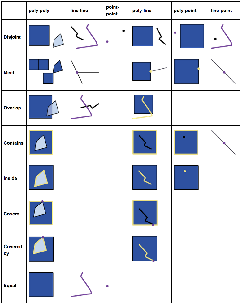
Dimensionally Extended nine-Intersection Model, aka DE-9IM,
describes the topological relations of two geometries in a plane.
With geometries a and b, operations I, B, E for interior, boundary and exterior,
operation dim for maximum dimension of a geometry, DE-9IM is defined as:
              ⎡ dim(I(a)∩I(b)) dim(I(a)∩B(b)) dim(I(a)∩E(b)) ⎤
DE9IM(a,b) =  ⎢ dim(B(a)∩I(b)) dim(B(a)∩B(b)) dim(B(a)∩E(b)) ⎥
              ⎣ dim(E(a)∩I(b)) dim(E(a)∩B(b)) dim(E(a)∩E(b)) ⎦
A spatial predicate is a test based on the DE-9IM. There are 10 relations that have a common name reflecting their semantics:
- Disjoint:
FF*FF****; - Intersects:
T********,*T*******,***T*****,****T****;- Covers:
T*****FF*,*T****FF*,***T**FF*,****T*FF*;- Contains:
T*****FF*;- Equals:
T*F**FFF*;
- Equals:
- Contains:
- CoveredBy:
T*F**F***,*TF**F***,**FT*F***,**F*TF***;- Within:
T*F**F***;
- Within:
- Touches:
FT*******,F**T*****,F***T****; - Crosses | dim(a)≠dim(b) or dim(any)=0:
T*T******,T*****T**,0********; - Overlaps | dim(a)=dim(b):
T*T***T**,1*T***T**;
- Covers:
† "Within" is sometimes known as "inside"; and "touches" as "meets".
Raster Data Analysis
Raster data analysis are mostly image processing (computational algebra).
Geo-Referencing
Aligning geographic data to a known coordinate system so it can be viewed, queried, and analyzed with other geographic data.
- shifting, rotating, scaling;
- skewing;
- warping, rubber sheeting;
- ortho-rectifying;
Filtering
Imagery (e.g. Lidar data):
- image band;
- histogram;
- change detection;
- classification (supervised/unsupervised): classify spectral signatures of features (vegetation, developed land, etc.);
- feature extraction;
- skeletonization: transform an image into its topological skeleton (e.g. by thining and trimming);
Interpolation
(spline, with tension, etc.)
Digital Elevation Model (DEM) Analysis
DEM data are stored in ASCII grids, which is a raster format.
- Terrain analysis (slope and aspect)
- Hillshade
- Hydrology: watersheds, flow lines
- Viewshed
- Flood inundation