Qualitative Theory of Differential Equations
Qualitative (or geometric) theory of ordinary differential equations, started by Henri Poincaré in 1881-1885, is the study of diffeomorphic invariants of the dynamical systems they represent. The phase space of second order ODEs is the Euclidean plane, the simplest manifold with nontrivial trajectories. Plane analysis of second order ODEs is the study of their fixed points and peoriodic orbits. Notes on qualitative theory of ODE, boundary value problem.
Fixed Point
Every linear first-order ODE system on the plane with a nonsingular coefficient matrix has a unique fixed point at the origin: $\dot y = A y$, $A \in \text{GL}(2, \mathbb{R})$. If the coefficient matrix has two real eigenvalues, e.g. $A = \text{diag}(\lambda_1, \lambda_2)$, then the ODE system has general solution: $y = \text{diag}(e^{\lambda_1 t}, e^{\lambda_2 t}) y_0$. If the coefficient matrix has a pair of complex eigenvalues, e.g. $A = \begin{pmatrix} a & b \\ -b & a \end{pmatrix}$, then the ODE system has general solution: $y_1 = c e^{at} \sin(bt+\phi)$, $y_2 = c e^{at} \cos(bt+\phi)$.
Linearization of an ODE system $\dot x = f(x)$: find fixed points, $f(x) = 0$; compute Jacobian matrix at the fixed points, $A = \nabla f(x_0)$; Jordan decompose the matrix, $A = P J P^{-1}$; solve the linear ODE system, $\dot \xi = J \xi$ where transformed coordinates $\xi = P^{-1} (x - x_0)$ and thus $x= P \xi - x_0$.
Node of a differentiable flow is a fixed point where the differential of the vector field has all positive or negative eigenvalues. Saddle is analogous to a node, but has both positive and negative eigenvalues and nothing else. Focus of a differentiable 2-dimensional flow is a fixed point where the differential of the vector field has a pair of complex eigenvalues with nonzero real parts. Every focus is topologically equivalent to a node. Center of a differentiable even-dimensional flow is a fixed point where the differential of the vector field has all purely imaginary nonzero eigenvalues. For linear systems, peoriodic orbits exist around a center and have the same period. For a nonlinear system, a center found in its linearized form may not be an actual center; but symmetry of the original system about y-axis suffice to preserve this property.

Figure: Topological classification of fixed points of dynamical systems on 2-manifolds.
Hyperbolicity in dynamical systems theory means nondegeneracy. Hyperbolic fixed point of a differentiable flow is a fixed point where the differential has no eigenvalues on the imaginary axis. A special case of hyperbolic flow corresponds to area-preserving vector fields on the plane, which have determinant one and the trajectories are the axes and standard hyperbolas $xy = c$, which is why such dynamical systems are called hyperbolic. Hyperbolic automorphism of a vector space is a bijiective linear transformation on the space with no eigenvalues on the complex unit circle: $T \in \text{GL}(V)$, $\sigma(T) \cap \mathbb{S}^1 = \emptyset$. The set of all hyperbolic automorphisms of a vector space is denoted by $\text{HL}(V)$. Hyperbolic fixed point of a differentiable cascade is a fixed point where the differential is a hyperbolic automorphism. Topological classification of hyperbolic fixed points: Differentiable flows on n-manifolds are locally topologically equivalent at hyperbolic fixed points if and only if the differentials of the vector fields at the fixed points have the same number of eigenvalues with negative (or positive) real parts; the theorem is analogous for differentiable cascades, but for their own differential, and is determined by the number of eigenvalues outside (or within) the complex unit circle.
Elliptic fixed point of a symplectic dynamical system is a fixed point where the differential of the Hamiltonian vector field has all purely imaginary nonzero eigenvalues. A large class of elliptic fixed points are Lyapunov stable.
Transverse fixed point of a differentiable flow is a fixed point where the differential of the vector field does not have eigenvalue zero. Transverse fixed point of a differentiable cascade is a fixed point where the graph intersects transversely with the diagonal: $(x, x) \in \Gamma{\psi} \pitchfork I$, where $I = \{(x, x) : x \in M\}$. A fixed point of a differentiable cascade is transverse if and only if the differential of the map at the point does not have eigenvalue one. Hyperbolic fixed points and elliptic fixed points are transverse.
Heteroclinic and Homoclinic Orbits
 Orbits of the Duffing equation
 Homoclinic orbits
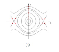
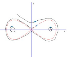
Heteroclinic orbit is a trajectory that connect two fixed points. Homoclinic orbit is a trajectory that connect the same fixed point. Homo- and hetero-clinic orbits typically approach the fixed points in infinite time, forward and backward, because in an eigenspace at a hyperbolic fixed point the solutions are exponential: $\dot y = \lambda y$, $y = e^{\lambda t}$. Duffing equation can be written as $\ddot{u} + u - u^3 = 0$; or as a first-order ODE system, $\begin{cases} \dot u = v \\ \dot v = -u + u^3 \end{cases}$. The duffing equation has a center at the origin and two saddles at $(\pm 1,0)$; it has heteroclinic orbits. The following system has homoclinic oribts: $\begin{cases} \dot x = y + y(1-x^2)[y^2-x^2(1-\frac{x^2}{2})] \\ \dot y = x(1-x^2) - y[y^2-x^2(1-\frac{x^2}{2})] \end{cases}$. It also has three fixed points: a saddle at the origin and two unstable foci at $(\pm 1,0)$.
Peoriodic Orbit
 Poincare-Bendixson theorem
First return function $\rho: U \mapsto \mathbb{R}$ for an open disc $Y$ transverse to a peoriodic orbit $\gamma_x$ in a dynamical system is the continuous real-valued function on a neighbourhood of the disc that gives the first time for every point in the neighbourhood to return to the disc: ${\phi(\rho(y), y) : y \in U} \subset Y$, $\rho(x) = \tau$ which is the period of the peoriodic orbit. Poincare map, first return map, or section map $f: U \mapsto Y$ for an open disc transverse to a peoriodic orbit in a dynamical system is the map that gives the location of first return for every point in a neighbourhood of the disc: $f(y) = \phi(\rho(y), y)$. The differential of a Poincare map is linearly conjugate the differential of the period-one transformation restricted to an invariant tangent hyperplane.
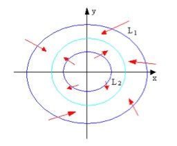
Limit cycle is a peoriodic orbit that any trajectory nearby either goes towards it, or moves away. Sink is a periodic orbit where all Lyapunov exponents are negative. Van der Pol equation has a sink. Poincare-Bendixson Theorem: For a planar dynamical system, if a ring-shaped region between two simple closed curves has no fixed point within, and any trajectory that intersects with the two boundary curves enters the region, then the region has at least one limit cycle. The conclusion holds if the inner boundary curve shrinks into an unstable node.
Hyperbolic peoriodic orbit in a dynamical system is a peoriodic orbit such that the differential of the transformation at one period of the orbit restricts to a hyperbolic automorphism on a tangent hyperplane at a point of the orbit: $T_x \phi^t = H \oplus \hat v_x \hat v_x^T$, $H \in \text{HL}(\mathbb{R}^{n-1})$, $\hat v_x = v_x / \|v_x\|$. A peoriodic orbit is hyperbolic if and only if a point on the orbit is a hyperbolic fixed point of a Poincare map at the point: $d f_x \in \text{HL}(\mathbb{R}^{n-1})$. Hyperbolic periodic point of a differentiable cascade is a periodic point where the differential of the period-one map is a hyperbolic automorphism: $T_x \phi^k \in \text{HL}(\mathbb{R}^n)$, where $k$ is the period. The orbit of a hyperbolic periodic point is called a hyperbolic periodic orbit.
Transverse periodic orbit of a differentiable flow is a fixed point where the differential of the period-one map has one as a simple eigenvalue; or equivalently, it is a transverse fixed point for a Poincare map.
Stability of Fixed Point
Local stability of fixed points of nonlinear dynamical systems can be defined in various ways. Lyapunov stable fixed point is one such that trajectories started near it stay nearby forever: [@Lyapunov1892] $\forall \varepsilon > 0$, $\exists \delta \in (0, \varepsilon)$: $d(x, x^∗ ) < \delta$ then $\sup_{t \ge 0} d(\phi_x(t), x^∗) < \varepsilon$.
(Locally) asymptotically stable fixed point is one that is Lyapunov stable and (locally) attractive, i.e. trajectories started near it converge to it: $\exists \delta > 0$: $d(x, x^∗) < \delta$ then $\lim_{t \to \infty} d(\phi_x(t), x^∗) = 0$. Notice that Lyapunov stability is distinct from local attractiveness. Basin of attraction or basin $B(x)$ of an asymptotically stable fixed point of a dynamical system is the union of all trajectories that tend toward the fixed point. Globally asymptotically stable fixed point is one that is Lyapunov stable and globally attractive, i.e. all trajectories converge to it.
Exponentially stable fixed point is one that is Lyapunov stable and (locally) exponentially attractive, i.e., trajectories started near it converge to it exponentially: $\exists \delta, \alpha, \beta > 0$: $d(x, x^∗) < \delta$ then $d(\phi_x(t), x^∗) / d(x, x^∗) \le \alpha e^{-\beta t}$.
Liapunov exponent...
Lyapunov function $V(x)$ for a differentiable flow with a fixed point at the origin is a locally positive-definite, continuously differentiable function with locally negative-semidefinite time derivative: $V \in C^1(\mathbb{R}^n, \mathbb{R}_{\ge 0})$; $V(x) = 0$ then $x = 0$; $\dot x = f(x)$, $(\nabla V, f) \le 0$. Lyapunov function is analogous to the energy of a dissipative physical system, but is not unique and thus easier to find. A fixed point is Lyapunov stable if and only if the dynamical system has a Lyapunov function. A fixed point is locally asymptotically stable if and only if the dynamical system has a Lyapunov function whose time derivative is locally negative-definite. A fixed point is globally asymptotically stable if the dynamical system has a radially unbounded global Lyapunov function whose time derivative is globally negative-definite.
Recurrence
Invariant Set
Global invariant set for a dynamical system is the subset $S$ of its state space whose orbits stay within itself: $\bigcup_{x \in S} \phi_x(G) \subset S$. Every fixed point or peoriodic orbit is a global invariant set. A dynamical system can be restricted to any of its global invariant sets. Local invariant set for a dynamical system is the subset of its state space whose local orbits stay within itself: $\exists t > 0$: $\bigcup_{x \in S} \phi_x([-t, t]) \subset S$. Local stable set $W^s_{\text{loc}}(x^∗)$ of a critical point is a subset of a neighborhood $U$ of the point where forward trajectories stay within and tend toward the point: $W^s_{\text{loc}}(x^∗) = \{x \in U : \phi_x([0, \infty)) \subset U, \lim_{t \to \infty} \phi_x(t) = x^∗\}$. Local unstable set is defined analogously but backwards: $W^u_{\text{loc}}(x^∗) = \{x \in U : \phi_x((-\infty, 0]) \subset U, \lim_{t \to -\infty} \phi_x(t) = x^∗\}$. [@Guckenheimer1983, p. 13]
Invariant subspace for a linear dynamical system is an invariant set such that it is a vector subspace $V$ of the state space. Stable, unstable, and center invariant subspaces $V^s, V^u, V^c$ of a linear dynamical system are the spans of the eigenspaces associated with eigenvalues that have negative, positive, and zero real parts, respectively.
Invariant manifold for a dynamical system is an invariant set that is a topological manifold as a topological subspace of the state space. Stable manifold $W^s$, or contracting manifold [@Arnold1973], is an invariant manifold where forward trajectories are bounded. Unstable manifold $W^u$, or dialating manifold, is analogously defined but backwards. Hadamard-Perron Theorem or stable-unstable manifold theorem for hyperbolic fixed point: For a hyperbolic fixed point of an autonomous dynamical system, its local stable and unstable invariant sets are submanifolds as smooth as the vector field, and their tangent spaces coincide with the stable and unstable invariant subspaces of the linearized dynamical system at the point: $T_x W^s_\text{loc}(x) = V^s(x)$; $f \in C^k$ then $W^s_\text{loc}(x) \in C^k$. Local stable manifold can be extended to a global stable manifold by flowing backwards, and analogously for local unstable manifold but forward: $W^s(x) = \bigcup_{t \le 0} \phi_t (W^s_\text{loc}(x))$. Global stable and unstable manifolds need not be submanifolds. Center manifold $W^c$ of a fixed point of a dynamical system is a local invariant manifold whose tangent space at the point is the center invariant subspace of the linearized dynamical system at the point. Center manifold theorem [@Guckenheimer and Holmes, 1983]: Every non-hyperbolic fixed point of a smooth dynamical system has a center manifold. Center manifold at a fixed point need not be unique.
Recurrence: Non-wandering Set
ω-limit set $\omega_x$ of a trajectory of a dynamical system is the set of limit points of all convergent subsequences of the forward trajectory: $\omega_x = \{\lim \phi_x(t_n) : \lim t_n = +\infty\}$; or equivalently, $\omega_x = \bigcap_{t \in \mathbb{R}} \overline{\phi_x([t, \infty))}$. α-limit set $\alpha_x$ is defined analogously but backwards. Recurrent point of a dynamical system is a point that belongs to its own ω-limit set: $\forall U(x)$, $\forall T > 0$, $\exists t > T$: $\phi(t, x) \in U$. Chain recurrent point...
Non-wandering point or nostalgic point of a dynamical system is a point such that: $\forall U(x)$, $\forall T > 0$, $\exists t > T$, $\exists y \in U$: $\phi(t, y) \in U$. Non-wandering set or Ω-set $\Omega(\phi)$ of a dynamical system is the set of all its non-wandering points. The non-wandering set of a dynamical system is a close invariant set, and it is non-empty if the phase space is compact. Topological conjugacies and equivalences preserve non-wandering sets.
Attracting set of a dynamical system is a closed invariant set that has a neighborhood where forward trajectories stay within and tend toward the invariant set: $\exists U(A)$: $\forall x \in U$, $\gamma_x^+ \subset U$, $\lim_{t\to\infty} d(\phi(t, x), A) = 0$. Repelling set is defined analogously but backwards.
Indecomposable closed invariant set is one where any point can be reached from any point by a finite number of forward transformations with arbitrarily small connecting distance: $\forall x, y \in A$, $\forall \varepsilon > 0$, $\exists (x_i)_{i=0}^n \subset X$, $\exists (t_i)_{i=0}^{n-1} \subset G_+$: $x_0 = x$, $d(\phi(t_i, x_i), x_{i+1}) < \varepsilon$, $x_n = y$. Attractor of a dynamical system is an indecomposable, closed, forward-invariant set whose every ε-neighborhood has a nonzero-volume subset whose forward trajectories are within the neighborhood and the ω-limit sets are within the invariant set [@Guckenheimer1983, Sec 1.6, 5.4]: $\forall \varepsilon > 0$, $\exists S \subset U_\varepsilon(A)$, $v(S) > 0$, $\bigcup_{x \in S} \gamma_x^+ \subset U_\varepsilon(A)$, $\bigcup_{x \in S} \omega_x \subset A$. Repellor is defined analogously but backwards. Attractor can be thought of as an attracting set that contains a dense orbit. Strange attractor is an attractor that includes a transverse homoclinic orbit.
Types of attractors:
- stable fixed point;
- periodic points: discrete periodic sequence;
- sink: attractive periodic trajectory;
- limit torus: periodic components with incommensurate frequencies;
- strange attractor: contains a transversal homoclinic orbit; with a fractal dimension;
periodic attractor. expanding attractor.
Nonlinear dynamical systems are typically chaotic. Notes on chaos
Stability of Dynamical System
Space of dynamical systems... C^s norm $\|\cdot\|_s$ of a $C^s$ vector field on a subset of a normed space is the maximum of the sup norms of the vector field and its partial derivatives up to order s: $v \in \mathfrak{X}^s(X)$, $\|v\|_s = \max_{|I| \le s} \left\|\frac{\partial v}{\partial x^I}\right\|_\infty$. C^s topology on a space of $C^s$ vector fields is the topology induced by the $C^s$ norm. Perturbation (摄动) of a $C^s$ vector field on a subset of a normed space is an element in a neighborhood of the vector field in the $C^s$-normed space of vector fields: $v' \in \mathfrak{X}^s(X)$, $\|v' -v\|_s < \varepsilon$.
Perturbation
Perturbation Theorem for fixed point: For every neighborhood of a regular singular point in a $C^1$ vector field, there is a neighborhood of the vector field where all vector fields in has a unique singular point in the neighborhood of the point: $v \in \mathfrak{X}^1(X)$, $v(x) = 0$, $d_x v \in \text{GL}(T_x X)$, $\forall U(x) \subset X$, $\exists U(v) \subset \mathfrak{X}^1(X)$: $\forall v' \in U(v)$, $\exists x' \in U(x)$, $v'(x') = 0$.
Perturbation method...
Averaging method...
Structural Stability
Structurally stable dynamical system is a dynamical system that is in the interior of its topological conjugacy/equivalence class: $f \in (C^r(X), \mathcal{T}_r)$, $\exists U(f)$: $U \subset [f]$.
Morse-Smale system is a dynamical system whose non-wandering set consists of a finite number of hyperbolic fixed points and hyperbolic peoriodic orbits, and it has no heteroclinic or homoclinic orbit. Theorem [@Peixoto1962]: A dynamical system on a compact orientable 2-manifold is $C^1$ structurally stable if and only if it is Morse-Smale; Morse-Smale systems are open and dense in $\mathfrak{X}^r(X)$. Theorem [@Palis and Smale, 1970]; Every Morse-Smale system on a compact manifold is $C^1$ structurally stable.
Anosov system... Theorem [@Anosov1962; @Anosov1967]: Every Anosov system on a compact manifold is $C^1$ structurally stable.
AS system is a dynamical system that satisfies Axiom A and the strong transversality condition. Theorem [@Robinson1974; @Robinson1976]: Every AS system is $C^1$ structurally stable.
C^0 density of C^1 structurally stable systems [@Smale1971; @Shub1972]: Every $C^r$ diffeomorphism on a compact manifold, $r \in \mathbb{N}_+$, is $C^r$ isotopic to a $C^1$ structurally stable system by an arbitrarily $C^0$-small isotopy.
Other definitions of stability of dynamical systems have also been introduced, the most interesting of which is Ω-stability. Ω-stable dynamical system is a dynamical system that is in the interior of its Ω-conjugacy/equivalence class: $f \in (C^r(X), \mathcal{T}_r)$, $\exists U(f)$: $U \subset [f|_\Omega]$. An Axiom A system on a compact manifold is Ω-stable if it has the no-cycle property.
Bifurcation
Bifurcation theory (分岔; branching) is the study of structural changes in a parametrized family of dynamical systems. Catastrophe theory is the application of bifurcation theory to the study of discontinuous or qualitative changes in long-term behavior of natural and social systems under varying external conditions.
Parametrized first-order ODE: $\dot x = f(x, \varepsilon)$
Local bifurcation... Global bifurcation...
Codimension-one bifurcation... Saddle-node bifurcation... Hopf bifurcation [@Hopf1943]... The periodic attractor shrinks until it merges with the unstable focus to form a stable focus.
Misc
Index of fixed point... Poincare-Hopf Theorem: The index sum of a flow on a compact manifold equals the Euler characteristic of the manifold.
Slow variable... Slow motion... Slow manifold...
References
- 王联、王慕秋, 非线性常微分方程定性分析. 哈工大出版社, 1987.
- 黄永念,非线性动力学讲义,2004.
- G. B. Whitham, Linear and Nonlinear Waves (1974).
- P Grindrod, Patterns and Waves (1991).
- J. Smoller, Shock Waves and Reaction Diffusion Equations (1994).