Qualitative Theory of Differential Equations
Types of Critical Points

Consider a linear 2nd-order ODE system, \[ \dot{\mathbf{y}} = B \mathbf{y} \] It may have one or a line of critical points, because unless \( B = 0 \), \( B \text{y} =0 \) has a unique solution or solutions forming a one-dimensional linear space. We assume \( \det(B) \ne 0 \) in the following discussion.

If \( B \) has real (nonzero) eigenvalues \( \lambda, \mu \), for example \( B = \begin{pmatrix} \lambda & 0 \\ 0 & \mu \end{pmatrix}\) , then \(\begin{cases} y_1 = y_1(0) e^{\lambda t} \\ y_2 = y_2(0) e^{\mu t} \end{cases}\).
- Source: \( \lambda, \mu > 0 \)
- Sink: \( \lambda, \mu < 0 \)
- Saddle: \( \lambda \mu < 0 \)

If \( B \) has a pair of complex conjugate eigenvalues \( a \pm ib \), for example \( B = \begin{pmatrix} a & b \\ -b & a \end{pmatrix} \) , then \(\begin{cases} y_1 = A e^{at} \sin(bt+\phi) \\ y_2 = A e^{at} \cos(bt+\phi) \end{cases}\)
- Unstable focus: \( a > 0 \)
- Stable focus: \( a < 0 \)
- Center: \( a = 0 \)
For linear systems, closed orbits exist around a center and have the same period. For a nonlinear system, a center found in its linearized form may not be an actual center; but symmetry of the original system about \(y\)-axis suffice to preserve this property.
Linearization at Critical Points
For a nonlinear 2nd-order ODE system: \[ \frac{\text{d}}{\text{d}t} \begin{pmatrix} x \\ y \end{pmatrix} = \begin{pmatrix} f(x,y) \\ g(x,y) \end{pmatrix} \]
- Find critical points: \( \begin{pmatrix} f(x_0,y_0) \\ g(x_0,y_0) \end{pmatrix} = 0 \)
- Linearize at the critical points: \( \frac{\text{d}}{\text{d}t} \begin{pmatrix} x \\ y \end{pmatrix} = \nabla\begin{pmatrix} f(x,y) \\ g(x,y) \end{pmatrix}\bigg\rvert_{(x_0,y_0)} \begin{pmatrix} x-x_0 \\ y-y_0 \end{pmatrix} + \text{h.o.t.} \)
- Switch axes to the critical point and get \( \frac{\text{d}}{\text{d}t} \begin{pmatrix} \tilde{x} \\ \tilde{y} \end{pmatrix} = A \begin{pmatrix} \tilde{x} \\ \tilde{y} \end{pmatrix}\) , where \(A\) is the Jacobian evaluated at the critical point.
- Normalize the coefficient matrix with \(P\), s.t. \( B= P^{-1}AP \) is a Jordan matrix.
- Solve the system w.r.t. \(P^{-1} \begin{pmatrix} \tilde{x} \\ \tilde{y} \end{pmatrix}\) as linearized cases.
To get the phase plane near a critical point, we just need a coordinate transformation, which does not change the eigenvalues of \(A\) and the type of the critical point.
If \( \mathbf{v} \) is an eigenvector corresponding to eigenvalue \( \lambda \) of the linearized system, along the line of the eigenvector we have \( \dot{x} = \lambda x \). This means along the eigenvectors at the critical point, trajectories go directly into or away from the critical point, approximately in a straight line.
Plane Analysis of 2nd-order Nonlinear ODE Systems
Duffing equation
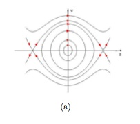 Trajectories in the Duffing equation
A form of Duffing equation is
\[ u'' + u - u^3 = 0 \]
Or, in the form of ODE systems,
\[ \begin{cases} u' = v \\ v' = -u+u^3 \end{cases} \]
We find three critical points: \( (0,0) \) and \( (\pm 1,0) \). Furthermore, the first one is a center, and the other two are saddles.
Heteroclinic & homoclinic orbits
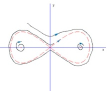 Homoclinic orbits
A trajectory may connect two critical points, or forms a loop from and toward the same critical point. The former one is called a heteroclinic orbit, and the latter a homoclinic orbit.
We've already seen heteroclinic orbits in duffing equation, now we illustrate a homoclinic oribt by the following system.
\[ \begin{cases} x' = y + y(1-x^2)[y^2-x^2(1-\frac{x^2}{2})] \\ y' = x(1-x^2) - y[y^2-x^2(1-\frac{x^2}{2})] \end{cases} \]
There are also three critical points: \( (0,0) \) and \( (\pm 1,0) \). The origin is a saddle, while the other two are unstable focus (foci).
Note: Period of homoclinic or heteroclinic orbit
- Generally, homoclinic and heteroclinic orbits go from and to saddle points. Since near saddle points, along the direction of eigenvectors, \( y'= \lambda y \), it takes infinite time to go to or leave the critical point.
- Hence, homo- and hetero-clinic orbits are typically with infinite period.
van der Pol equation
Van der Pol equation has an attracting limit cycle.
Limit cycle
 The Poincare-Bendixon theorem and limit cycle
A limit cycle is a closed orbit that each trajectory nearby either goes towards it, or leaves away. It is another important type of closed orbits.
Certain theorems guarantee the existence of a limit cycle.
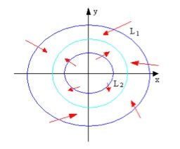
Poincare-Bendixon Theorem:
- Assume that \(B\) is a ring-shaped domain between two simple closed curves \(L_1\) and \(L_2\). There is no critical point in this domain. Moreover, any trajectory that intersects with these two curves enters \(B\). Then there exist at least one limit cycle in this domain.
- The conclusion holds if the inner boundary curve \(L_2\) shrinks into an unstable node.
Stability and Lyapunov Function
Hierarchy of local stabilities in nonlinear dynamical systems:
- An equilibrium is Lyapunov stable {Lyapunov1892} if trajectories started near it stay nearby forever: \[ \forall \varepsilon > 0, \exists \delta \in (0, \varepsilon): d( x(0), x^* ) < \delta \Rightarrow \sup_{t \ge 0} d(x(t), x^*) < \varepsilon \]
- An equilibrium is asymptotically stable if it is Lyapunov stable and (locally) attractive, that is, trajectories started near it converge to it: \[ \exists \delta > 0: d( x(0), x^* ) < \delta \Rightarrow \lim_{t \to +\infty} d(x(t), x^*) = 0 \]
- An equilibrium is exponentially stable if it is Lyapunov stable and (locally) exponentially attractive, that is , trajectories started near it converge to it exponentially: \[ \exists \delta, \alpha, \beta > 0: d( x(0), x^* ) < \delta \Rightarrow d( x(t), x^* ) / d( x(0), x^* ) \le \alpha e^{-\beta t} \]
Notice that Lyapunov stability is distinct from local attractiveness.
An equilibrium is globally asymptotically stable if it is Lyapunov stable and globally attractive, that is, all trajectories converge to it.
A Lyapunov function \( V(\mathbf{x}) \) for an autonomous dynamical system \( \dot{\mathbf{x}} = \mathbf{g}(\mathbf{x}) \) with an equilibrium point at the origin is a locally positive-definite and continuously differentiable function such that its time derivative is locally negative-semidefinite:
- \( V \in C^1(\mathbb{R}^n, \mathbb{R}) \)
- \( V(\mathbf{x}) > 0, \forall x \ne 0 \), \( V(0) = 0 \)
- \( \nabla V \cdot \mathbf{g}(\mathbf{x}) \le 0, \forall x \ne 0 \)
An equilibrium is Lyapunov stable if and only if the dynamical system has a Lyapunov function. An equilibrium is locally asymptotically stable if and only if the dynamical system has a Lyapunov function whose time derivative is locally negative-definite. An equilibrium is globally asymptotically stable if the dynamical system has a radially unbounded global Lyapunov function whose time derivative is globally negative-definite.
Lyapunov function is analogous to the energy of a dissipative physical system, while not unique and thus easier to find.
Bifurcation Theory
A subset of the phase space is an attractor if it is the smallest subset of itself that is forward invariant and has a basin of attraction: \( \Phi(A, t) \subseteq A, \forall t > 0 \); and \( \exists B \in \tau(X), B \supseteq A\), \( \forall b \in B, \forall \varepsilon > 0, \exists T > 0: \Phi(b, t) \in N_\varepsilon(A), \forall t > T \).
Types of attractors:
- stable fixed point (sink, stable focus)
- periodic points: discrete periodic sequence
- limit cycle: periodic trajectory
- limit torus: periodic components with incommensurate frequencies
- strange attractor: attractors with a fractal dimension
The ω-limit set of a trajectory \( \Phi(x, t) \) of a dynamical system is the set of limit points of all convergent subsequences of the forward trajectory: \( \Omega_x = \{ \omega \mid \exists \{t_k\}, \lim_{k \to \infty} t_k = +\infty, \lim_{k \to \infty} \Phi(x, t_k) = \omega \} \).
Chaos
References
- 王联、王慕秋, 非线性常微分方程定性分析. 哈工大出版社,1987.
- 黄永念,非线性动力学讲义,2004.
- J. Smoller, Shock Waves and Reaction Diffusion Equations, Springer (1994)
- P Grindrod, Patterns and Waves, Claredon, 1991
- G. B. Whitham, Linear and Nonlinear Waves, John Wiley & Sons (1974).