Qualitative Theory of Differential Equations
Types of Critical Points

Consider a linear 2nd-order ODE system, $$\dot{\mathbf{y}} = B \mathbf{y}$$ It may have one or a line of critical points, because unless $B = 0$, $B \text{y} =0$ has a unique solution or solutions forming a one-dimensional vector space. We assume $\det(B) \ne 0$ in the following discussion.

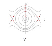
If $B$ has real (nonzero) eigenvalues $\lambda, \mu$, for example $B = \begin{pmatrix} \lambda & 0 \\ 0 & \mu \end{pmatrix}$, then $\begin{cases} y_1 = y_1(0) e^{\lambda t} \\ y_2 = y_2(0) e^{\mu t} \end{cases}$.
- Source: $\lambda, \mu > 0$
- Sink: $\lambda, \mu < 0$
- Saddle: $\lambda \mu < 0$

If $B$ has a pair of complex conjugate eigenvalues $a \pm ib$, for example $B = \begin{pmatrix} a & b \\ -b & a \end{pmatrix}$ , then $\begin{cases} y_1 = A e^{at} \sin(bt+\phi) \\ y_2 = A e^{at} \cos(bt+\phi) \end{cases}$
- Unstable focus: $a > 0$
- Stable focus: $a < 0$
- Center: $a = 0$
For linear systems, closed orbits exist around a center and have the same period. For a nonlinear system, a center found in its linearized form may not be an actual center; but symmetry of the original system about y-axis suffice to preserve this property.
Linearization at Critical Points
For a nonlinear 2nd-order ODE system: $$\frac{\text{d}}{\text{d}t} \begin{pmatrix} x \\ y \end{pmatrix} = \begin{pmatrix} f(x,y) \\ g(x,y) \end{pmatrix}$$
- Find critical points: $\begin{pmatrix} f(x_0,y_0) \\ g(x_0,y_0) \end{pmatrix} = 0$
- Linearize at the critical points: $\frac{\text{d}}{\text{d}t} \begin{pmatrix} x \\ y \end{pmatrix} = \nabla\begin{pmatrix} f(x,y) \\ g(x,y) \end{pmatrix}\bigg\rvert_{(x_0,y_0)} \begin{pmatrix} x-x_0 \\ y-y_0 \end{pmatrix} + \text{h.o.t.}$
- Switch axes to the critical point and get $\frac{\text{d}}{\text{d}t} \begin{pmatrix} \tilde{x} \\ \tilde{y} \end{pmatrix} = A \begin{pmatrix} \tilde{x} \\ \tilde{y} \end{pmatrix}$, where $A$ is the Jacobian evaluated at the critical point.
- Normalize the coefficient matrix with $P$, s.t. $B= P^{-1}AP$ is a Jordan matrix.
- Solve the system w.r.t. $P^{-1} \begin{pmatrix} \tilde{x} \\ \tilde{y} \end{pmatrix}$ as linearized cases.
To get the phase plane near a critical point, we just need a coordinate transformation, which does not change the eigenvalues of $A$ and the type of the critical point.
If $\mathbf{v}$ is an eigenvector corresponding to eigenvalue $\lambda$ of the linearized system, along the line of the eigenvector we have $\dot{x} = \lambda x$. This means along the eigenvectors at the critical point, trajectories go directly into or away from the critical point, approximately in a straight line.
Plane Analysis of 2nd-order Nonlinear ODE Systems
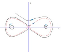
Duffing equation
 Trajectories in the Duffing equation
A form of Duffing equation is $$u'' + u - u^3 = 0$$ Or, in the form of ODE systems, $$\begin{cases} u' = v \\ v' = -u+u^3 \end{cases}$$
We find three critical points: $(0,0)$ and $(\pm 1,0)$. Furthermore, the first one is a center, and the other two are saddles.
Heteroclinic & homoclinic orbits
 Homoclinic orbits
A trajectory may connect two critical points, or forms a loop from and toward the same critical point. The former one is called a heteroclinic orbit, and the latter a homoclinic orbit.
We've already seen heteroclinic orbits in duffing equation, now we illustrate a homoclinic oribt by the following system.
$$\begin{cases} x' = y + y(1-x^2)[y^2-x^2(1-\frac{x^2}{2})] \\ y' = x(1-x^2) - y[y^2-x^2(1-\frac{x^2}{2})] \end{cases}$$
There are also three critical points: $(0,0)$ and $(\pm 1,0)$. The origin is a saddle, while the other two are unstable focus (foci).
Note: Period of homoclinic or heteroclinic orbit
- Generally, homoclinic and heteroclinic orbits go from and to saddle points. Since near saddle points, along the direction of eigenvectors, $y'= \lambda y$, it takes infinite time to go to or leave the critical point.
- Hence, homo- and hetero-clinic orbits are typically with infinite period.
van der Pol equation
Van der Pol equation has an attracting limit cycle.
Limit cycle
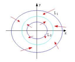 The Poincare-Bendixson theorem and limit cycle
A limit cycle is a closed orbit that any trajectory nearby either goes towards it, or moves away. It is another important type of closed orbits.
Poincare-Bendixson Theorem: For a planar dynamical system, if a ring-shaped region between two simple closed curves has no critical point within, and any trajectory that intersects with the two boundary curves enters the region, then the region has at least one limit cycle. The conclusion holds if the inner boundary curve shrinks into an unstable node.
Stability and Lyapunov Function
Hierarchy of local stabilities in nonlinear dynamical systems:
- An equilibrium is Lyapunov stable [@Lyapunov1892] if trajectories started near it stay nearby forever: $$\forall \varepsilon > 0, \exists \delta \in (0, \varepsilon): d( x(0), x^∗ ) < \delta \Rightarrow \sup_{t \ge 0} d(x(t), x^∗) < \varepsilon$$
- An equilibrium is asymptotically stable if it is Lyapunov stable and (locally) attractive, that is, trajectories started near it converge to it: $$\exists \delta > 0: d( x(0), x^∗ ) < \delta \Rightarrow \lim_{t \to +\infty} d(x(t), x^∗) = 0$$
- An equilibrium is exponentially stable if it is Lyapunov stable and (locally) exponentially attractive, that is, trajectories started near it converge to it exponentially: $$\exists \delta, \alpha, \beta > 0: d( x(0), x^∗ ) < \delta \Rightarrow d( x(t), x^∗ ) / d( x(0), x^∗ ) \le \alpha e^{-\beta t}$$
Notice that Lyapunov stability is distinct from local attractiveness.
An equilibrium is globally asymptotically stable if it is Lyapunov stable and globally attractive, that is, all trajectories converge to it.
A Lyapunov function $V(\mathbf{x})$ for an autonomous dynamical system $\dot{\mathbf{x}} = \mathbf{g}(\mathbf{x})$ with an equilibrium point at the origin is a locally positive-definite and continuously differentiable function such that its time derivative is locally negative-semidefinite:
- $V \in C^1(\mathbb{R}^n, \mathbb{R})$
- $V(\mathbf{x}) > 0, \forall x \ne 0$, $V(0) = 0$
- $\nabla V \cdot \mathbf{g}(\mathbf{x}) \le 0, \forall x \ne 0$
An equilibrium is Lyapunov stable if and only if the dynamical system has a Lyapunov function. An equilibrium is locally asymptotically stable if and only if the dynamical system has a Lyapunov function whose time derivative is locally negative-definite. An equilibrium is globally asymptotically stable if the dynamical system has a radially unbounded global Lyapunov function whose time derivative is globally negative-definite.
Lyapunov function is analogous to the energy of a dissipative physical system, while not unique and thus easier to find.
Bifurcation Theory
A subset of the phase space is an attractor if it is the smallest subset of itself that is forward invariant and has a basin of attraction: $\Phi(A, t) \subseteq A, \forall t > 0$; and $\exists B \in \tau(X), B \supseteq A$, $\forall b \in B, \forall \varepsilon > 0, \exists T > 0: \Phi(b, t) \in N_\varepsilon(A), \forall t > T$.
Types of attractors:
- stable fixed point (sink, stable focus)
- periodic points: discrete periodic sequence
- limit cycle: periodic trajectory
- limit torus: periodic components with incommensurate frequencies
- strange attractor: attractors with a fractal dimension
The ω-limit set of a trajectory $\Phi(x, t)$ of a dynamical system is the set of limit points of all convergent subsequences of the forward trajectory: $\Omega_x = \{ \omega \mid \exists \{t_k\}, \lim_{k \to \infty} t_k = +\infty, \lim_{k \to \infty} \Phi(x, t_k) = \omega \}$.
Chaos
References
- 王联、王慕秋, 非线性常微分方程定性分析. 哈工大出版社,1987.
- 黄永念,非线性动力学讲义,2004.
- J. Smoller, Shock Waves and Reaction Diffusion Equations, Springer (1994)
- P Grindrod, Patterns and Waves, Claredon, 1991
- G. B. Whitham, Linear and Nonlinear Waves, John Wiley & Sons (1974).