Random Process
Basic Descriptions of Random Processes (Chap 12.1)
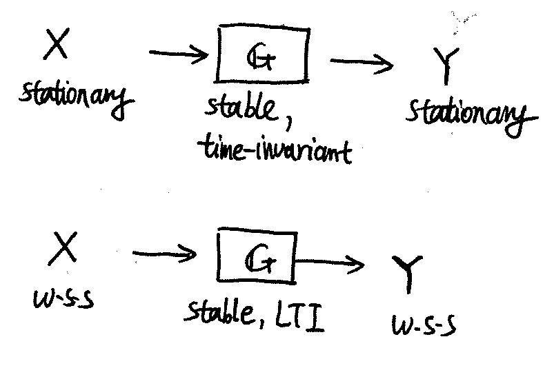
- \( X(u,t) \) is W.S.S., \( \iff m_X, \text{and } R_X(\tau) / k_X(\tau) / S_X(\tau) \).
- \( R(t_1,t_2) \) is a covariance function, iff it is Hermitian, positive semi-definite.

Two views of stochastic process
A number of procedures have been proposed for the canonical representations of general stochastic processes. Two views are listed below:
- Discrete sample (measurements) approaching a continuous signal. \( X: \Omega\times D \to \mathbb{R} \)
- Function space as the range probability space. \( X: \Omega \to H \)
Random field (RF)
Random field is a measurable function on a product space, where one of the subdomains is a probability space, to the real line.
Symbolically, random field \( \alpha: D\times \Omega \to \mathbb{R} \) is a \( (\mathcal{S} \times \Sigma, \mathcal{B}) \)-measurable or \( ( (\mathcal{S} \times \Sigma)^* , \mathcal{L} ) \)-measurable function. Here \( (D, \mathcal{S}, \mu) \) is a deterministic measure space, and \( (\Omega, \Sigma, P) \) is a probability space. Their product space is \( ( D \times \Omega, \mathcal{S} \times \Sigma, \mu \times P) \), with completion \( ( D \times \Omega, (\mathcal{S} \times \Sigma)^{*}, \mu \times P) \). Either Borel measure or Lebesgue measure is applied to the real line.
Think of the deterministic field \(D\) as an index set. When \(D\) is finite, the RF can be seen as a random vector, i.e. a finite collection of random variables, or a random sample. When the number of samples approaches infinity, the RF can be seen as a random sequence. When \(D\) is a space with power of the continuum, e.g. the real line or an Euclidean space, the RF is often seen as a general random process.
Given an undirected graph \(G=(V,E)\), a set of random variables \( X = {X_v}, v\in V \) form a Markov random field (MRF) with respect to \(G\) if they satisfy the local Markov properties: \( P(X_i = x_i \mid X_j = x_j, j = V \setminus \{i\}) = P(X_i = x_i \mid X_j = x_j, j = \partial_i) \).
A Gibbs random field (GRF) is a set of random variables that if all degrees of freedom outside an arbitrary subset are frozen, the canonical ensemble for the subset subject to these boundary conditions matches the probabilities in the Gibbs measure conditional on the frozen degrees of freedom: \( P(X=x) = \frac{1}{Z(\beta)} \exp ( - \beta E(x)) \).
The fundamental theorem of random fields (Hammersley–Clifford theorem): [@Hammersley1971] Given an undirected graph, any positive probability measure with the Markov properties is a Gibbs measure for some locally-defined energy function.
Random process (RP)
Gaussian process is a real random process, of which all finite-dimensional distributions are Gaussian. That is, for any finite collection of instances \( t_1, \dots, t_n \in T \), the characteristic function of random vector \( (X(t_1), \dots, X(t_n)) \) has the form \( \phi(u_1, \dots, u_n; t_1, \dots, t_n) = \exp{ i \sum_k A(t_k) u_k - \frac{1}{2} \sum_{k,j} B(t_k, t_j) u_k u_j } \), where \(A(t)\) is the mathematical expectation and \(B(t, s)\) is the covariance function. Gaussian processes can be seen as an infinite-dimensional generalization of multivariate Gaussian distributions. Gaussian processes are useful in statistical modelling for its analytical convenience.
Power Spectral Density
(Chap. 14.2, 15.1)
- \( S_X(f) = \mathcal{F}{ R_X(\tau) } \), assumming \( X(u,t) \) W.S.S.
- \( R_X(0) = P_X = \int_{\mathbb{R}} S_X(f) \mathrm{d} f \)
- \( S_X(f) \geq 0, x \in \mathbb{R} \), then \( S_X(f) \) is an even function.
- \( X(u,t), Y(u,t) \) are uncorrelated and \( Z=X+Y \), then \( S_Z(f) = S_X(f) + S_Y(f) \)
- \( S_{XY^* } (f) = \mathcal{F}{ R_{XY^* } (\tau) } \), assumming \( X(u,t), Y(u,t) \) jointly W.S.S.
- \( S_X(f) \) does not consist of Dirac delta functions, only if \( m_X =0 \);