Random Process
Stochastic processes can be represented from (at least) two perspectives:
- Discrete sample/measurements approaching a continuous signal: $X: \Omega\times D \to \mathbb{R}$;
- Function space as the range probability space: $X: \Omega \to H$;
Random Field
Random field (RF) is a measurable function on a product space, where one of the subdomains is a probability space, to the real line.
Symbolically, random field $\alpha: D\times \Omega \to \mathbb{R}$ is a $(\mathcal{S} \times \Sigma, \mathcal{B})$-measurable or $( (\mathcal{S} \times \Sigma)^∗ , \mathcal{L} )$-measurable function. Here $(D, \mathcal{S}, \mu)$ is a deterministic measure space, and $(\Omega, \Sigma, P)$ is a probability space. Their product space is $( D \times \Omega, \mathcal{S} \times \Sigma, \mu \times P)$, with completion $( D \times \Omega, (\mathcal{S} \times \Sigma)^{*}, \mu \times P)$. Either Borel measure or Lebesgue measure is applied to the real line.
Think of the deterministic field $D$ as an index set. When $D$ is finite, the RF can be seen as a random vector, i.e. a finite collection of random variables, or a random sample. When the number of samples approaches infinity, the RF can be seen as a random sequence. When $D$ is a space with power of the continuum, e.g. the real line or a Euclidean space, the RF is often seen as a general random process.
Given an undirected graph $G=(V,E)$, a set of random variables $X = {X_v}, v\in V$ form a Markov random field (MRF) with respect to $G$ if they satisfy the local Markov properties: $P(X_i = x_i \mid X_j = x_j, j = V \setminus \{i\}) = P(X_i = x_i \mid X_j = x_j, j = \partial_i)$.
Gibbs random field (GRF) is a set of random variables that if all degrees of freedom outside an arbitrary subset are frozen, the canonical ensemble for the subset subject to these boundary conditions matches the probabilities in the Gibbs measure conditional on the frozen degrees of freedom: $P(X=x) = \frac{1}{Z(\beta)} \exp ( - \beta E(x))$.
Fundamental theorem of random fields (Hammersley–Clifford theorem): [@Hammersley1971] Given an undirected graph, any positive probability measure with the Markov properties is a Gibbs measure for some locally-defined energy function.
Random Process
Random Process (RP).
Ito process (named after Kiyosi Itô) is a stochastic process with a stochastic differential. More specifically, an Ito process w.r.t. a non-decreasing family of sigma-algebras on the underlying set of a probability space is a random process on the non-negative real line whose stochastic differential can be written as an Ito stochastic differential equation (ISDE) of the form: $\text{d} \mathbf{x} = \mathbf{a}~\text{d} t + \mathbf{b}~\text{d} \mathbf{w}$, where $\mathbf{w}_t$ is a Wiener process w.r.t. $(\Sigma_t)_{t \ge 0}$, $\mathbf{a}_t$ and $\mathbf{b}_t$ are random processes measurable w.r.t. $\Sigma_t$ for each $t$, and $\forall t \le t'$, $\Sigma_t \subset \Sigma_{t'}$. For a real-valued function $f(x, t): \mathbb{R}^n \times \mathbb{R}_{\ge 0} \mapsto \mathbb{R}$ such that $\frac{\partial^2 f}{\partial x^2}$ and $\frac{\partial f}{\partial t}$ are continuous, given an Ito process $\mathbf{x}_t$, the random process $f(\mathbf{x}_t, t)$ is a diffusion process whose stochastic differential can be computed by the Ito formula aka Ito's lemma [@Ito1951]: $\text{d} \mathbf{f} = \left( \frac{\partial f}{\partial t} + \mathbf{a} \frac{\partial f}{\partial x} + \frac{\mathbf{b}^2}{2} \frac{\partial^2 f}{\partial x^2} \right) \text{d} t + \mathbf{b} \frac{\partial f}{\partial x}~\text{d} \mathbf{w}$.
Markov Process
Markov process is a random process on a subset of the real line such that it satisfies the Markov property, i.e. the distribution of any future state conditional on the entire state history is the same as that conditional on the present state: $(\mathbf{x}_t)_{t \in T}$, $\forall t, t' \in T, t < t'$, $\mathbf{x}_{t'} \mid (\mathbf{x}_u)_{u \le t} \sim \mathbf{x}_{t'} \mid \mathbf{x}_t$. Markov jump process is Markov process with a continuous index set and a discrete state space. Markov chain is a Markov process with a discrete index set.
Feller process is a homogeneous Markov process on an additive sub-semi-group of the real line, whose transition function maps continuous bounded functions to continuous functions [@Feller1952]: $\forall f \in (C(X), \|\cdot\|_\infty)$, $\forall t \in T$, $P^t f \in C(X)$, where $x \in (X, \mathcal{T}, \mathcal{B})$, $P: T \times X \times \mathcal{B} \mapsto \mathbb{R}_{\ge 0}$, and $P^t f(x) = \int_X f(y) P(t, x, \mathrm{d}y)$. Infinitesimal generator of a Feller process is an operator defined as: $\mathcal{L} f(x) = \lim_{t \to 0+} \frac{P^t f(x) - f(x)}{t}$. The infinitesimal generator and the transition function of a Feller process are related by: $P^t f(x) = e^{t \mathcal{L}} f(x)$. The generator of a diffusion process is: $\mathcal{L} = a \cdot \nabla + \frac{1}{2} \langle b b^T, \nabla^2 \rangle_F$. The generator of the Wiener process is half the Laplacian operator, $\frac{1}{2} \Delta$.
Diffusion process is a Markov process on the non-negative real line that satisfies an ISDE of the form: $\text{d} \mathbf{x} = a(\mathbf{x}, t)~\text{d} t + b(\mathbf{x}, t)~\text{d} \mathbf{w}$, where $x \in \mathbb{R}^n$, $t \in [0, \infty)$, $\mathbf{w}$ is the m-dimensional Wiener process, drift coefficient $a(x, t) \in \mathbb{R}^n$, and diffusion coefficient $b^2(x, t) \in M_{n,m}(\mathbb{R})$. In other words, a diffusion process is an Ito process that is Markovian: $\mathbf{a}_t = a(\mathbf{x}, t)$ and $\mathbf{b}_t = b(\mathbf{x}, t)$. Brownian motion is a diffusion process with constant drift and diffusion coefficient: for $a(x, t) = \mu$ and $b^2(x, t) = \sigma^2$, $\mathbf{x}_t = \mu t + \sigma \mathbf{w}_t$, where $\mathbf{w}_t$ is the Wiener process. Geometric Brownian motion is a diffusion process whose drift coefficient and the square root of diffusion coefficient are linear in state and constant in time: $a(x, t) = \mu x$, $b(x, t) = \sigma x$.
Gaussian Process
Gaussian process is a real random process whose finite subsets are all Gaussian random vectors: $(\mathbf{x}_t)_{t \in T}$, $\forall A \subset T, |A| \in \mathbb{N_+}$, random vector $(\mathbf{x}_t)_{t \in A}$ has characteristic function $\phi(u) = \exp( i \sum_{j \in A} m(j) u_j - \frac{1}{2} \sum_{j,k \in A} C(j, k) u_j u_k)$. Gaussian processes can be seen as infinite-dimensional generalizations of Gaussian random vectors. and are easy to analyze.
Wiener process $(\mathbf{w}_t)_{t \in \mathbb{R}_{\ge 0}}$ is a Gaussian process on the non-negative real line, with mean zero and covariance function equal to the smaller index: $m(t) = 0$, and $C(s, t) = \min(s, t)$. The Wiener process is a Markov process, and is the basis for diffusion processes. Sampling the Wiener process at any increasing sequence of indices, each term equals its predecessor plus an independent zero-mean Gaussian random variable whose variance equals the time gap (the predecessor of the first term is always zero): $\mathbf{x}_{t_1} \sim N(0, t_1)$; $\mathbf{x}_{t_{k+1}} = \mathbf{x}_{t_k} + \sqrt{t_{k+1} - t_k} \mathbf{z}$, where $\mathbf{z} \sim N(0, 1)$.
Empirical Process
Empirical process is a random process from the underlying set $X$ of a random variable $(X, Σ, P)$ to the scaled deviation of the empirical measure $P_n$, i.e. a random function: $\mathcal{G}(x) = \sqrt{n} (F_n(x) - F(x))$. The (classical) empirical process can be generalized to the sigma-algebra $Σ$ or classes of measurable functions ${f: (X, Σ) \mapsto (\mathbb{R}, \mathcal{B(T_d)})}$. Empirical processes are used to prove propositions uniform in the underlying set, esp. Glivenko–Cantelli theorems (uniform laws of large numbers), laws of the iterated logarithm, central limit theorems, and probability inequalities. For certain classes (Vapnik–Chervonenkis, Donsker) of the underlying set, the empirical process converges weakly to a Gaussian process, as sample size tends to infinity.
Second-order Random Processes
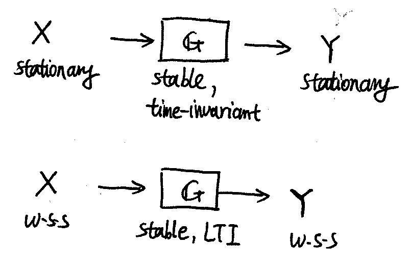
Description of a second-order random process [@Scholtz2013, Chap 3.2, 12.1]. Wide-sense stationary (WSS) random process is one whose second-order description is translation-invariant: $m_x(t) = m_x(t + t')$, $K_x(t_1, t_2) = K_x(t_1 + t', t_2 + t')$; equivalently, the covariance function can be substituted with the correlation function $R_x(t_1, t_2)$, or power spectral density $S_x$.
Power spectral density (Chap. 14.2, 15.1):
- $S_X(f) = \mathcal{F}{ R_X(\tau) }$, assumming $X(u,t)$ W.S.S.
- $R_X(0) = P_X = \int_{\mathbb{R}} S_X(f) \mathrm{d} f$
- $S_X(f) \geq 0, x \in \mathbb{R}$, then $S_X(f)$ is an even function.
- $X(u,t), Y(u,t)$ are uncorrelated and $Z=X+Y$, then $S_Z(f) = S_X(f) + S_Y(f)$
- $S_{XY^∗ } (f) = \mathcal{F}{ R_{XY^∗ } (\tau) }$, assumming $X(u,t), Y(u,t)$ jointly W.S.S.
- $S_X(f)$ does not consist of Dirac delta functions, only if $m_X =0$;