Spectral Analysis
This article summarizes spectral analysis.
Power Spectral Density
Theoretical preparation to spectral density estimation: Random-Process#power-spectral-density
Intensities over a frequency spectrum (such as power spectral density) is often plot on logarithmic scales, reflecting the dynamic range (ratio of the maximum and the minimum) of spectral components. Some common log scale units: decade is a factor of 10, octave is a factor of 2; 10 decibels (dB) is 1 decade. Octave is such named because a frequency band with dynamic range 2 is called an octave (纯八度) in music, where the eighth note (音符) denotes a harmonic twice the frequency of the first. Given a reference value, these dimensionless units become absolute units. For signal power, decibel watt (dBW) and decibel milliwatt (dBm) take watt (W) and milliwatt (mW) as reference value respectively.
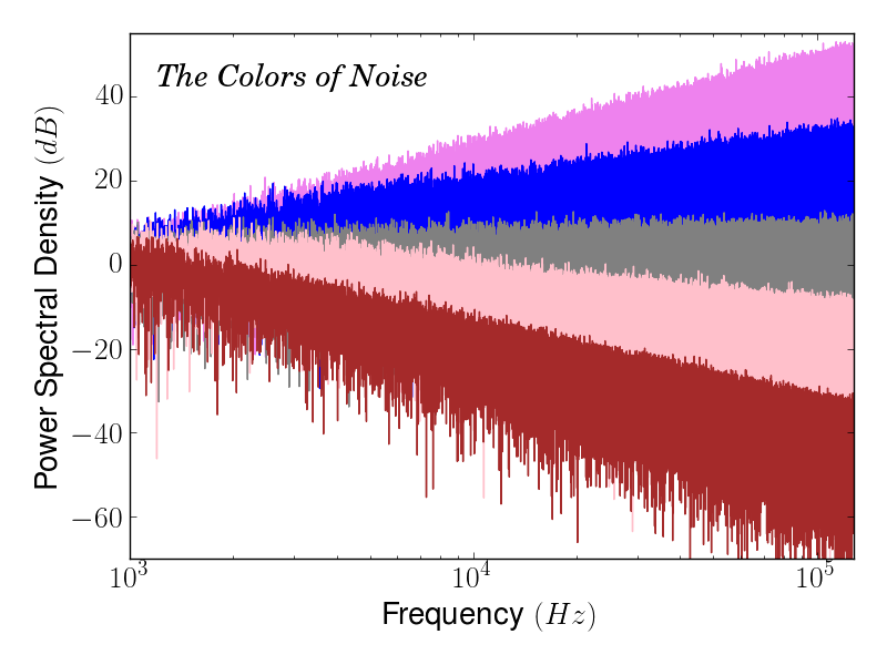
White noise is a random signal with power uniformly distributed over the frequency spectrum. In general, power-law noise is a random signal with power spectral density being a power-law function, $S_X(f) = f^{\beta}$. On log-log scale, power spectral density of a power-law noise is linear, with slope $\beta$ (or $10 \beta$ in dB/decade). Power-law noise with specific values of $\beta$ have color names: -1 for pink noise, -2 for brown/Brownian noise; 1 for blue noise, 2 for violet noise. The color names correspond to the apparent color if the random signal is an electromagnetic wave on the visible spectrum. All power-law noises are theoretical models, because actual signals can never have a frequency spectrum of infinite dynamic range.
Spectral Density Estimation
Spectral density estimation is estimating the power spectral density of a random signal from a time-series sample.
 Figure: A voice waveform over time and its broad power spectrum.
Spectral analysis involves a trade-off between resolving comparable strength components with similar frequencies and resolving disparate strength components with dissimilar frequencies. The following explains the cause and trade-off strategy in detail.
Sampling
Sampling: the reduction of a continuous signal to a discrete signal, typically equal-spaced in time.
- Sample rate: frequency of time series $f_s$.
- DFT sample frequency: sample rate divided by the number of DFT bins (typically equal to the sample length/count; preferably integer powers of 2).
- Nyquist frequency (folding frequency): half sample rate; DFT spectrum folds and repeats its segment between zero and the Nyquist frequency.
Aliasing (effect of sampling on the frequency spectrum): periodic repetition of the entire spectrum.
 Figure: continuous Fourier transform, Fourier transform of periodic summation, discrete time Fourier transform (DTFT), and discrete Fourier transform (DFT). Notice that sampling always introduces periodic spectral repetition.
Windowing
Window function: a function of finite support that gets multiplied with a waveform before estimating its spectral density (on a finite time interval).
Spectral leakage (effects of windowing on the frequency spectrum): Windowing causes the true spectrum S(f) to be convoluted with the Fourier transform of the window function F{w}.
- Equivalent noise bandwidth (ENBW): width of the lobes (rectangular shapes) the DTFT redistributed into.
- Noise floor: power spectrum of the window function averaged over time, forming the base of a frequency spectrum, height (compared to the physical noise floor) proportional to ENBW.
- Scalloping loss: the reduced power spectral density when a spectral component is not a multiple of the DFT sample frequency, with maximum loss equal to the power spectrum of the window function at half ENBW (compared to value at zero).
Choice of window function for spectral density estimation:
- rectangular window has the smallest spectral leakage but wide noise floor(?), good for analyzing a transient signal, harmonic content/distortion;
- high dynamic range (wideband applications)
 Figure: Comparison of window functions.
